2. 🐍 Introduction to Python: Basic Libraries for AI



1 Introduction
📌 What You Will Learn:
Fundamental Python programming concepts
Introduction to NumPy and Pandas for data handling
Basics of data visualization using Matplotlib
Practical exercises tailored to surgical task analysis
🎯 Goal:
By the end of this notebook, you will have a solid foundation in Python and be able to load, manipulate, and analyze surgical motion data, preparing you for more advanced machine learning tasks.
Let’s get started! 🚀
2 NumPy
NumPy provides an in depth overview of what exactly NumPy is. Quoting them: >At the core of the NumPy package, is the ndarray object. This encapsulates n-dimensional arrays of homogeneous data types, with many operations being performed in compiled code for performance.
Let’s get started by importing it, typically shortened to np because of how frequently it’s called. This will come standard in most Python distributions such as Anaconda. If you need to install it simply: ~~~ !pip install numpy ~~~
[1]:
import numpy as np
Creating Arrays
Manually or from Lists
Manually create a list and demonstrate that operations on that list are difficult.
[2]:
lst = [0, 1, 2, 3]
lst * 2
[2]:
[0, 1, 2, 3, 0, 1, 2, 3]
That isn’t what we expected! For lists, we need to loop through all elements to apply a function to them which can be incredibly time consuming.
[3]:
[i * 2 for i in lst]
[3]:
[0, 2, 4, 6]
Now lets make a numpy array and once in an array, let’s show how intuitive operations are now that they are performed element by element.
[4]:
array = np.array(lst)
print(array)
print(array * 2)
print(array + 2)
[0 1 2 3]
[0 2 4 6]
[2 3 4 5]
Let’s create a 2D matrix of 32 bit floats.
[5]:
np.array([[1, 0, 0],
          [0, 1, 0],
          [0, 0, 1]], dtype=np.float32)
[5]:
array([[1., 0., 0.],
       [0., 1., 0.],
       [0., 0., 1.]], dtype=float32)
Using Functions
We’ll go through a few here, but for more in depth examples and options see NumPy’s Array Creation Routines. These first few examples are for very basic arrays/matrices.
[6]:
np.zeros(5)
[6]:
array([0., 0., 0., 0., 0.])
[7]:
np.zeros([2, 3])
[7]:
array([[0., 0., 0.],
       [0., 0., 0.]])
[8]:
np.eye(3)
[8]:
array([[1., 0., 0.],
       [0., 1., 0.],
       [0., 0., 1.]])
Now let’s start making sequences.
[9]:
np.arange(10)
[9]:
array([0, 1, 2, 3, 4, 5, 6, 7, 8, 9])
[10]:
np.arange(0,  #start
          10) #stop (not included in array)
[10]:
array([0, 1, 2, 3, 4, 5, 6, 7, 8, 9])
[11]:
np.arange(0,  #start
          10, #stop (not included in array)
          2)  #step size
[11]:
array([0, 2, 4, 6, 8])
[12]:
np.linspace(0,  #start
            10, #stop (default to be included, can pass in endpoint=False)
            6)  #number of data points evenly spaced
[12]:
array([ 0., 2., 4., 6., 8., 10.])
[13]:
np.logspace(0, #output starts being raised to this value
            3, #ending raised value
            4) #number of data points
[13]:
array([ 1., 10., 100., 1000.])
Logspace is the equivalent of rasing a base by a linspaced array.
[14]:
10 ** np.linspace(0,3,4)
[14]:
array([ 1., 10., 100., 1000.])
[15]:
np.logspace(0, 4, 5, base=2)
[15]:
array([ 1., 2., 4., 8., 16.])
If you don’t want to have to do the mental math to know what exponent to raise the values to, you can use geomspace but this only helps for base of 10.
[16]:
np.geomspace(1, 1000, 4)
[16]:
array([ 1., 10., 100., 1000.])
Random numbers!
[17]:
np.random.rand(5)
[17]:
array([0.10419445, 0.72301424, 0.92475581, 0.82504997, 0.09006971])
[18]:
np.random.rand(2, 3)
[18]:
array([[0.91349968, 0.80744317, 0.41486676],
       [0.69650334, 0.3682823 , 0.55498108]])
Indexing
Let’s first create a simple array.
[19]:
array = np.arange(1, 11, 1)
array
[19]:
array([ 1, 2, 3, 4, 5, 6, 7, 8, 9, 10])
Now index the first item.
[20]:
array[0]
[20]:
np.int64(1)
Index the last item.
[21]:
array[-1]
[21]:
np.int64(10)
Grab every 2nd item.
[22]:
array[::2]
[22]:
array([1, 3, 5, 7, 9])
Grab every second item starting at index of 1 (the second value)
[23]:
array[1::2]
[23]:
array([ 2, 4, 6, 8, 10])
Start from the second item, going to the 7th but skipping every other. (Our first time using the full array[start (inclusive): stop (exclusive): step] array ‘slicing’ notation)
[24]:
array[1:6:2]
[24]:
array([2, 4, 6])
Reverse the order.
[25]:
array[::-1]
[25]:
array([10, 9, 8, 7, 6, 5, 4, 3, 2, 1])
Boolean operations to index the array.
[26]:
array[array < 5]
[26]:
array([1, 2, 3, 4])
[27]:
array[array * 2 < 5]
[27]:
array([1, 2])
Integer list can also index arrays.
[28]:
array[[1,3,5]]
[28]:
array([2, 4, 6])
Now let’s create a slightly more complicated, 2 dimensional array.
[29]:
array_2d = np.arange(10).reshape((2, 5))
array_2d
[29]:
array([[0, 1, 2, 3, 4],
       [5, 6, 7, 8, 9]])
Indexing the second dimension.
[30]:
array_2d[:, 1]
[30]:
array([1, 6])
Any combination of these indexing methods works as well.
[31]:
array_2d[[True, False], 1::2]
[31]:
array([[1, 3]])
[32]:
array_2d[1, [0,1,4]]
[32]:
array([5, 6, 9])
Operations
[33]:
array
[33]:
array([ 1, 2, 3, 4, 5, 6, 7, 8, 9, 10])
[34]:
array + 100
[34]:
array([101, 102, 103, 104, 105, 106, 107, 108, 109, 110])
[35]:
array * 2
[35]:
array([ 2, 4, 6, 8, 10, 12, 14, 16, 18, 20])
To raise all the elements in an array to an exponent we have to use the notation ** not ^.
[36]:
array ** 2
[36]:
array([ 1, 4, 9, 16, 25, 36, 49, 64, 81, 100])
Use that shape to create a new array matching it to do operations with.
[37]:
array2 = np.arange(array.shape[0]) * 5
array2
[37]:
array([ 0, 5, 10, 15, 20, 25, 30, 35, 40, 45])
[38]:
array2 + array
[38]:
array([ 1, 7, 13, 19, 25, 31, 37, 43, 49, 55])
Stats of an Array
[39]:
print(array)
print(array_2d)
[ 1  2  3  4  5  6  7  8  9 10]
[[0 1 2 3 4]
 [5 6 7 8 9]]
[40]:
print(array.shape)
print(array_2d.shape)
(10,)
(2, 5)
[41]:
print(len(array))
print(len(array_2d))
10
2
[42]:
print(array.max())
print(array_2d.max())
10
9
[43]:
print(array.min())
print(array_2d.min())
1
0
[44]:
array.std()
[44]:
np.float64(2.8722813232690143)
[45]:
array.cumsum()
[45]:
array([ 1, 3, 6, 10, 15, 21, 28, 36, 45, 55])
[46]:
array.cumprod()
[46]:
array([      1,       2,       6,      24,     120,     720,    5040,
         40320,  362880, 3628800])
Constants
[47]:
np.pi
[47]:
3.141592653589793
[48]:
np.e
[48]:
2.718281828459045
[49]:
np.inf
[49]:
inf
Functions
[50]:
np.sin(np.pi / 2)
[50]:
np.float64(1.0)
[51]:
np.cos(np.pi)
[51]:
np.float64(-1.0)
[52]:
np.log(np.e)
[52]:
np.float64(1.0)
[53]:
np.log10(100)
[53]:
np.float64(2.0)
[54]:
np.log2(64)
[54]:
np.float64(6.0)
To demonstrate rounding, let’s first make a new array with decimals.
[55]:
array = np.arange(4) / 3
print(array)
np.around(array, 2)
[0. 0.33333333 0.66666667 1. ]
[55]:
array([0. , 0.33, 0.67, 1. ])
Looping vs Vectorization
As mentioned in the beginning, NumPy uses machine code with their ndarray objects which is what leads to the performance improvements. Let’s demonstrate this by constructing a simple sine wave.
[56]:
fs = 500 #sampling rate in Hz
d_t = 1 / fs #time steps in seconds
n_step = 1000 #number of steps (there will be n_step+1 data points)

amp = 1 #amplitude of sine wave
f = 2 #frequency of sine wave

time = np.linspace(0,             #start time
                   n_step * d_t,    #end time
                   num=n_step + 1)  #number of data points, one more than the steps to include an endpoint
time.shape
[56]:
(1001,)
First we make a function to loop through each element and calculate the amplitude.
[57]:
def sine_wave_with_loop(time, amp, f, phase=0):
  length = time.shape[0]
  wave = np.zeros(length)

  for i in range(length-1):
    wave[i] = np.sin(2 * np.pi * f * time[i] + phase * np.pi / 180)*amp
  return wave
Now let’s time how quickly that executes for our time array of 1,001 data points.
[58]:
%timeit sine_wave_with_loop(time, amp, f)
1.41 ms ± 306 μs per loop (mean ± std. dev. of 7 runs, 1,000 loops each)
Now let’s do the same using NumPy’s sine function and vectorization.
[59]:
def sine_wave_with_numpy(time, amp, f, phase=0):
  """Takes in a time array and sine wave parameters, returns an array of the sine wave amplitude."""
  return np.sin(2 * np.pi * f * time + phase * np.pi / 180) * amp
Notice my docstrings!
[60]:
help(sine_wave_with_numpy)
Help on function sine_wave_with_numpy in module __main__:

sine_wave_with_numpy(time, amp, f, phase=0)
    Takes in a time array and sine wave parameters, returns an array of the sine wave amplitude.
[61]:
%timeit sine_wave_with_numpy(time, amp, f)
17.2 μs ± 3.68 μs per loop (mean ± std. dev. of 7 runs, 100,000 loops each)
Using vectorization is about 100x faster! And this increases the longer the loops are.
Why Vectorization Works So Much Faster
The above example highlights that NumPy is much faster, but why? Because it is using compiled machine code under the hood for it’s operations.
Python has the Numba package which can be used to do this compilation which we will do to highlight just why NumPy is faster (and recommended!).
[62]:
from numba import njit

numba_sine_wave_with_loop = njit(sine_wave_with_loop)
numba_sine_wave_with_numpy = njit(sine_wave_with_numpy)
[63]:
%timeit numba_sine_wave_with_loop(time, amp, f)
%timeit numba_sine_wave_with_numpy(time, amp, f)
The slowest run took 5.39 times longer than the fastest. This could mean that an intermediate result is being cached.
21.3 μs ± 19.4 μs per loop (mean ± std. dev. of 7 runs, 1 loop each)
The slowest run took 4.73 times longer than the fastest. This could mean that an intermediate result is being cached.
23.7 μs ± 18 μs per loop (mean ± std. dev. of 7 runs, 1 loop each)
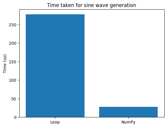
Let’s combine this into a DataFrame we’ll discuss next in more detail, but here’s a preview.
[64]:
import pandas as pd

time_data = pd.DataFrame({'Time (us)':[2.77*100, 27.5, 23.1, 22.6],
                          'Method':['Loop','NumPy','Loop','NumPy'],
                          'Numba?':['w/o','w/o','w','w']}
)
time_data
[64]:
| Time (us) | Method | Numba? | |
|---|---|---|---|
| 0 | 277.0 | Loop | w/o |
| 1 | 27.5 | NumPy | w/o |
| 2 | 23.1 | Loop | w |
| 3 | 22.6 | NumPy | w |
Now let’s plot it and preview Plotly!
[65]:
import matplotlib.pyplot as plt

fig = plt.bar(time_data['Method'], time_data['Time (us)'])
plt.ylabel('Time (us)')
plt.title('Time taken for sine wave generation')

plt.show()
3 Pandas
Pandas is built on top of NumPy meaning that the data is stored still as NumPy ndarray objects under the hood. But it exposes a much more intuitive labeling/indexing architecture and allows you to link arrays of different types (strings, floats, integers etc.) to one another.
To quote Jake VanderPlas: >At the very basic level, Pandas objects can be thought of as enhanced versions of NumPy structured arrays in which the rows and columns are identified with labels rather than simple integer indices.
To start, import pandas as pd, again this will come standard in virtually all Python distributions such as Anaconda. But to install is simply: ~~~ !pip install pandas ~~~
[66]:
import pandas as pd
There are three types of Pandas objects, we’ll only focus on the first two: 1. Series – 1D labeled homogeneous array, sizeimmutable 2. Data Frames – 2D labeled, size-mutable tabular structure with heterogenic columns 3. Panel – 3D labeled size mutable array.
Creating a Series
First let’s create a few numpy arrays.
[67]:
amplitude = sine_wave_with_numpy(time, amp, f, 180)
print(time)
print(amplitude)
[0.    0.002 0.004 ... 1.996 1.998 2.   ]
[ 1.22464680e-16 -2.51300954e-02 -5.02443182e-02 ...  5.02443182e-02
  2.51300954e-02  1.10218212e-15]
Now let’s see what a series looks like made from one of the arrays.
[68]:
pd.Series(amplitude)
[68]:
0       1.224647e-16
1      -2.513010e-02
2      -5.024432e-02
3      -7.532681e-02
4      -1.003617e-01
            ...
996     1.003617e-01
997     7.532681e-02
998     5.024432e-02
999     2.513010e-02
1000    1.102182e-15
Length: 1001, dtype: float64
This type of series has some value, but you really start to see it when you add in an index.
[69]:
series = pd.Series(data=amplitude,
                   index=time,
                   name='Amplitude')
series
[69]:
0.000    1.224647e-16
0.002   -2.513010e-02
0.004   -5.024432e-02
0.006   -7.532681e-02
0.008   -1.003617e-01
             ...
1.992    1.003617e-01
1.994    7.532681e-02
1.996    5.024432e-02
1.998    2.513010e-02
2.000    1.102182e-15
Name: Amplitude, Length: 1001, dtype: float64
Here’s where Pandas shines - indexing is much more intuitive (and inclusive) to specify based on labels, not those confusing integer locations. We’ll come back to this when we have the dataframe next too.
[70]:
series[0: 0.01]
[70]:
0.000    1.224647e-16
0.002   -2.513010e-02
0.004   -5.024432e-02
0.006   -7.532681e-02
0.008   -1.003617e-01
0.010   -1.253332e-01
Name: Amplitude, dtype: float64
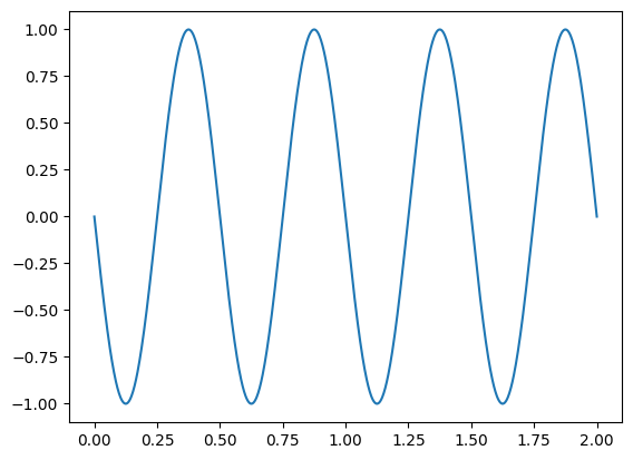
Being able to plot quickly is also a plus!
[71]:
series.plot()
[71]:
<Axes: >
Remember we never left the NumPy array, it is still here and can be accessed with the following.
[72]:
series.values
[72]:
array([ 1.22464680e-16, -2.51300954e-02, -5.02443182e-02, ...,
        5.02443182e-02,  2.51300954e-02,  1.10218212e-15])
[73]:
series.to_numpy()
[73]:
array([ 1.22464680e-16, -2.51300954e-02, -5.02443182e-02, ...,
        5.02443182e-02,  2.51300954e-02,  1.10218212e-15])
Creating a DataFrame
A DataFrame is basically a sequence of aligned series objects, and by aligned I mean they share a common index or label. This let’s us mix and match types easily among other benefits.
First we’ll start creating dataframes using what is called a “dictionary” with keys and values.
[74]:
df = pd.DataFrame({"Phase 0": sine_wave_with_numpy(time, amp, f, 00),
                   "Phase 90": sine_wave_with_numpy(time, amp, f, 90),
                   "Phase 180": sine_wave_with_numpy(time, amp, f, 180),
                   "Phase 270": sine_wave_with_numpy(time, amp, f, 270)},
                  index=time)
df
[74]:
| Phase 0 | Phase 90 | Phase 180 | Phase 270 | |
|---|---|---|---|---|
| 0.000 | 0.000000e+00 | 1.000000 | 1.224647e-16 | -1.000000 |
| 0.002 | 2.513010e-02 | 0.999684 | -2.513010e-02 | -0.999684 |
| 0.004 | 5.024432e-02 | 0.998737 | -5.024432e-02 | -0.998737 |
| 0.006 | 7.532681e-02 | 0.997159 | -7.532681e-02 | -0.997159 |
| 0.008 | 1.003617e-01 | 0.994951 | -1.003617e-01 | -0.994951 |
| ... | ... | ... | ... | ... |
| 1.992 | -1.003617e-01 | 0.994951 | 1.003617e-01 | -0.994951 |
| 1.994 | -7.532681e-02 | 0.997159 | 7.532681e-02 | -0.997159 |
| 1.996 | -5.024432e-02 | 0.998737 | 5.024432e-02 | -0.998737 |
| 1.998 | -2.513010e-02 | 0.999684 | 2.513010e-02 | -0.999684 |
| 2.000 | -9.797174e-16 | 1.000000 | 1.102182e-15 | -1.000000 |
1001 rows × 4 columns
Plotting (Preview)
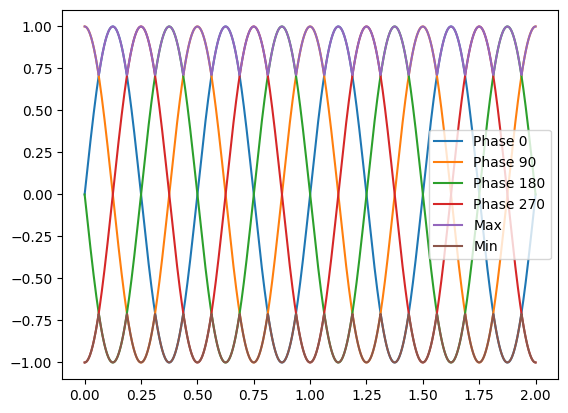
Dataframes also wrap around Matplotlib to allow for plotting directly from the dataframe object itself. This can also be done from the Pandas Series object too like we showed earlier.
[75]:
df.plot()
[75]:
<Axes: >

[76]:
df['Max'] = df.max(axis=1)
df['Min'] = df.min(axis=1)
df
[76]:
| Phase 0 | Phase 90 | Phase 180 | Phase 270 | Max | Min | |
|---|---|---|---|---|---|---|
| 0.000 | 0.000000e+00 | 1.000000 | 1.224647e-16 | -1.000000 | 1.000000 | -1.000000 |
| 0.002 | 2.513010e-02 | 0.999684 | -2.513010e-02 | -0.999684 | 0.999684 | -0.999684 |
| 0.004 | 5.024432e-02 | 0.998737 | -5.024432e-02 | -0.998737 | 0.998737 | -0.998737 |
| 0.006 | 7.532681e-02 | 0.997159 | -7.532681e-02 | -0.997159 | 0.997159 | -0.997159 |
| 0.008 | 1.003617e-01 | 0.994951 | -1.003617e-01 | -0.994951 | 0.994951 | -0.994951 |
| ... | ... | ... | ... | ... | ... | ... |
| 1.992 | -1.003617e-01 | 0.994951 | 1.003617e-01 | -0.994951 | 0.994951 | -0.994951 |
| 1.994 | -7.532681e-02 | 0.997159 | 7.532681e-02 | -0.997159 | 0.997159 | -0.997159 |
| 1.996 | -5.024432e-02 | 0.998737 | 5.024432e-02 | -0.998737 | 0.998737 | -0.998737 |
| 1.998 | -2.513010e-02 | 0.999684 | 2.513010e-02 | -0.999684 | 0.999684 | -0.999684 |
| 2.000 | -9.797174e-16 | 1.000000 | 1.102182e-15 | -1.000000 | 1.000000 | -1.000000 |
1001 rows × 6 columns
This will be the topic of the next webinar, plotting with Plotly!
Note that I need to install an upgraded version of Plotly in Colab because the default Plotly Express version doesn’t work in Colab (but their more advanced graph objects does).
[77]:
import matplotlib.pyplot as plt
[78]:
fig, ax = plt.subplots()
df.plot(ax=ax)
plt.show()
Load from CSV
This dataset was discussed in a blog on vibration metrics and used bearing data as an example.
Note you don’t have to use a CSV. They have a lot of other file formats natively supported (see full list): * hdf * feather * pickle
But I know everyone likes CSVs!
[79]:
df = pd.read_csv('https://info.endaq.com/hubfs/Plots/bearing_data.csv', index_col=0)
df
[79]:
| Fault_021 | Fault_014 | Fault_007 | Normal | |
|---|---|---|---|---|
| Time | ||||
| 0.000000 | -0.105351 | -0.074395 | 0.053116 | 0.046104 |
| 0.000083 | 0.132888 | 0.056365 | 0.116628 | -0.037134 |
| 0.000167 | -0.056535 | 0.201257 | 0.083654 | -0.089496 |
| 0.000250 | -0.193178 | -0.024528 | -0.026477 | -0.084906 |
| 0.000333 | 0.064879 | -0.072284 | 0.045319 | -0.038594 |
| ... | ... | ... | ... | ... |
| 9.999667 | 0.095754 | 0.145055 | -0.098923 | 0.064254 |
| 9.999750 | -0.123083 | 0.092263 | -0.067573 | 0.070721 |
| 9.999833 | -0.036508 | -0.168120 | 0.005685 | 0.103265 |
| 9.999917 | 0.097006 | -0.035898 | 0.093400 | 0.124335 |
| 10.000000 | -0.008762 | 0.165846 | 0.130923 | 0.114947 |
120000 rows × 4 columns
Save CSV
Like reading data, there are a host of native formats we can save data from a dataframe. See documentation.
[80]:
df.to_csv('bearing-data.csv')
Simple Analysis
[81]:
df.describe()
[81]:
| Fault_021 | Fault_014 | Fault_007 | Normal | |
|---|---|---|---|---|
| count | 120000.000000 | 120000.000000 | 120000.000000 | 120000.000000 |
| mean | 0.012251 | 0.002729 | 0.002953 | 0.010755 |
| std | 0.198383 | 0.157761 | 0.121272 | 0.065060 |
| min | -1.037862 | -1.338628 | -0.650390 | -0.269114 |
| 25% | -0.107020 | -0.096649 | -0.072284 | -0.032544 |
| 50% | 0.011682 | 0.001299 | 0.004548 | 0.013351 |
| 75% | 0.132054 | 0.100872 | 0.080081 | 0.056535 |
| max | 0.917908 | 1.124376 | 0.594025 | 0.251382 |
[82]:
df.std()
[82]:
Fault_021    0.198383
Fault_014    0.157761
Fault_007    0.121272
Normal       0.065060
dtype: float64
[83]:
df.max()
[83]:
Fault_021    0.917908
Fault_014    1.124376
Fault_007    0.594025
Normal       0.251382
dtype: float64
Note that these built in Pandas functions are using NumPy to process and are the equivalent of doing the following.
[84]:
np.max(df)
[84]:
np.float64(1.124375968063872)
[85]:
df.quantile(0.25)
[85]:
Fault_021   -0.107020
Fault_014   -0.096649
Fault_007   -0.072284
Normal      -0.032544
Name: 0.25, dtype: float64
[86]:
df['abs(max)'] = df.abs().max(axis=1)
df
[86]:
| Fault_021 | Fault_014 | Fault_007 | Normal | abs(max) | |
|---|---|---|---|---|---|
| Time | |||||
| 0.000000 | -0.105351 | -0.074395 | 0.053116 | 0.046104 | 0.105351 |
| 0.000083 | 0.132888 | 0.056365 | 0.116628 | -0.037134 | 0.132888 |
| 0.000167 | -0.056535 | 0.201257 | 0.083654 | -0.089496 | 0.201257 |
| 0.000250 | -0.193178 | -0.024528 | -0.026477 | -0.084906 | 0.193178 |
| 0.000333 | 0.064879 | -0.072284 | 0.045319 | -0.038594 | 0.072284 |
| ... | ... | ... | ... | ... | ... |
| 9.999667 | 0.095754 | 0.145055 | -0.098923 | 0.064254 | 0.145055 |
| 9.999750 | -0.123083 | 0.092263 | -0.067573 | 0.070721 | 0.123083 |
| 9.999833 | -0.036508 | -0.168120 | 0.005685 | 0.103265 | 0.168120 |
| 9.999917 | 0.097006 | -0.035898 | 0.093400 | 0.124335 | 0.124335 |
| 10.000000 | -0.008762 | 0.165846 | 0.130923 | 0.114947 | 0.165846 |
120000 rows × 5 columns
Indexing
Here is where indexing in Python gets a whole lot more intuitive! A dataframe with an index let’s use index values (time in this case) to slice the dataframe, not rely on the nth element in the arrays.
[87]:
df[0: 0.05]
[87]:
| Fault_021 | Fault_014 | Fault_007 | Normal | abs(max) | |
|---|---|---|---|---|---|
| Time | |||||
| 0.000000 | -0.105351 | -0.074395 | 0.053116 | 0.046104 | 0.105351 |
| 0.000083 | 0.132888 | 0.056365 | 0.116628 | -0.037134 | 0.132888 |
| 0.000167 | -0.056535 | 0.201257 | 0.083654 | -0.089496 | 0.201257 |
| 0.000250 | -0.193178 | -0.024528 | -0.026477 | -0.084906 | 0.193178 |
| 0.000333 | 0.064879 | -0.072284 | 0.045319 | -0.038594 | 0.072284 |
| ... | ... | ... | ... | ... | ... |
| 0.049584 | 0.131010 | 0.129136 | -0.014619 | 0.021487 | 0.131010 |
| 0.049667 | 0.437675 | -0.221399 | -0.025340 | 0.021070 | 0.437675 |
| 0.049750 | 0.095754 | -0.120689 | 0.033137 | 0.035256 | 0.120689 |
| 0.049834 | -0.137269 | 0.275977 | 0.023716 | 0.044226 | 0.275977 |
| 0.049917 | 0.150203 | 0.019167 | -0.044670 | 0.005424 | 0.150203 |
600 rows × 5 columns
We can also use the same convention as before by adding in a step definition, in this case we’ll grab every 100th point.
[88]:
df[0: 0.05: 100]
[88]:
| Fault_021 | Fault_014 | Fault_007 | Normal | abs(max) | |
|---|---|---|---|---|---|
| Time | |||||
| 0.000000 | -0.105351 | -0.074395 | 0.053116 | 0.046104 | 0.105351 |
| 0.008333 | -0.481067 | -0.137745 | -0.010558 | -0.012934 | 0.481067 |
| 0.016667 | -0.265985 | -0.073746 | -0.140669 | 0.027329 | 0.265985 |
| 0.025000 | -0.192343 | 0.203856 | -0.168120 | -0.029832 | 0.203856 |
| 0.033334 | 0.018984 | 0.154476 | -0.072933 | 0.076353 | 0.154476 |
| 0.041667 | -0.289975 | -0.227409 | 0.088202 | 0.016898 | 0.289975 |
There are ways to use the integer based indexing if you so desire.
[89]:
df.iloc[0:10]
[89]:
| Fault_021 | Fault_014 | Fault_007 | Normal | abs(max) | |
|---|---|---|---|---|---|
| Time | |||||
| 0.000000 | -0.105351 | -0.074395 | 0.053116 | 0.046104 | 0.105351 |
| 0.000083 | 0.132888 | 0.056365 | 0.116628 | -0.037134 | 0.132888 |
| 0.000167 | -0.056535 | 0.201257 | 0.083654 | -0.089496 | 0.201257 |
| 0.000250 | -0.193178 | -0.024528 | -0.026477 | -0.084906 | 0.193178 |
| 0.000333 | 0.064879 | -0.072284 | 0.045319 | -0.038594 | 0.072284 |
| 0.000417 | 0.214874 | 0.034761 | 0.060751 | 0.025451 | 0.214874 |
| 0.000500 | -0.076353 | 0.094212 | -0.174130 | 0.040680 | 0.174130 |
| 0.000583 | -0.065922 | -0.070010 | -0.229521 | 0.042558 | 0.229521 |
| 0.000667 | 0.206529 | -0.079431 | 0.045482 | 0.038177 | 0.206529 |
| 0.000750 | 0.021487 | 0.092426 | 0.027452 | 0.044018 | 0.092426 |
Rolling
I love the rolling method which allows for easy rolling window calculations, something you’ll do frequently with time series data.
[90]:
n = int(df.shape[0] / 100)
df.rolling(n).max()
[90]:
| Fault_021 | Fault_014 | Fault_007 | Normal | abs(max) | |
|---|---|---|---|---|---|
| Time | |||||
| 0.000000 | NaN | NaN | NaN | NaN | NaN |
| 0.000083 | NaN | NaN | NaN | NaN | NaN |
| 0.000167 | NaN | NaN | NaN | NaN | NaN |
| 0.000250 | NaN | NaN | NaN | NaN | NaN |
| 0.000333 | NaN | NaN | NaN | NaN | NaN |
| ... | ... | ... | ... | ... | ... |
| 9.999667 | 0.748721 | 0.768318 | 0.408362 | 0.18525 | 0.933137 |
| 9.999750 | 0.748721 | 0.768318 | 0.408362 | 0.18525 | 0.933137 |
| 9.999833 | 0.748721 | 0.768318 | 0.408362 | 0.18525 | 0.933137 |
| 9.999917 | 0.748721 | 0.768318 | 0.408362 | 0.18525 | 0.933137 |
| 10.000000 | 0.748721 | 0.768318 | 0.408362 | 0.18525 | 0.933137 |
120000 rows × 5 columns
[91]:
df.rolling(n).max()[::n]
[91]:
| Fault_021 | Fault_014 | Fault_007 | Normal | abs(max) | |
|---|---|---|---|---|---|
| Time | |||||
| 0.000000 | NaN | NaN | NaN | NaN | NaN |
| 0.100001 | 0.726190 | 0.710166 | 0.443448 | 0.184416 | 0.813809 |
| 0.200002 | 0.696150 | 0.641131 | 0.411773 | 0.204443 | 0.740376 |
| 0.300003 | 0.491289 | 0.846612 | 0.492178 | 0.172525 | 0.846612 |
| 0.400003 | 0.578699 | 0.608482 | 0.524828 | 0.204860 | 0.608482 |
| ... | ... | ... | ... | ... | ... |
| 9.500079 | 0.731823 | 0.500950 | 0.474798 | 0.206112 | 0.760820 |
| 9.600080 | 0.697818 | 0.713253 | 0.470412 | 0.190466 | 0.713253 |
| 9.700081 | 0.677791 | 0.547244 | 0.415996 | 0.229060 | 0.677791 |
| 9.800082 | 0.625220 | 0.569498 | 0.391469 | 0.176489 | 0.653801 |
| 9.900083 | 0.749555 | 0.949271 | 0.332342 | 0.176489 | 0.949271 |
100 rows × 5 columns
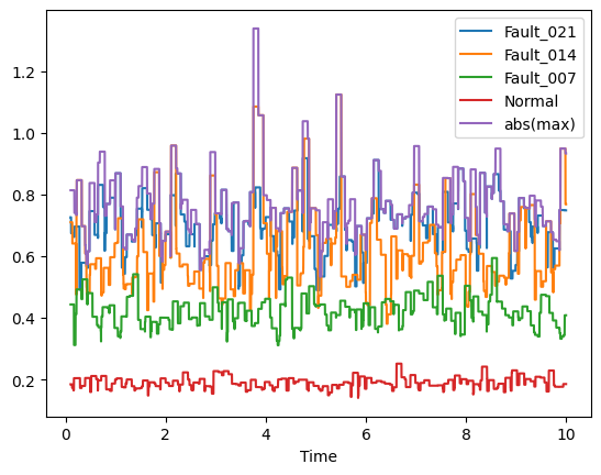
[92]:
df.rolling(n).max().plot()
[92]:
<Axes: xlabel='Time'>
Datetime Data (Yay Finance!)
Let’s use Yahoo Finance and stock data as a relatable example of data with datetimes.
[93]:
%pip install -q yfinance
import yfinance as yf
Note: you may need to restart the kernel to use updated packages.
[94]:
df =  yf.download(["SPY", "AAPL", "MSFT", "AMZN", "GOOGL"],
                  start='2019-01-01',
                  end='2021-09-24')
df
YF.download() has changed argument auto_adjust default to True
[*********************100%***********************] 5 of 5 completed
[94]:
| Price | Close | High | ... | Open | Volume | ||||||||||||||||
|---|---|---|---|---|---|---|---|---|---|---|---|---|---|---|---|---|---|---|---|---|---|
| Ticker | AAPL | AMZN | GOOGL | MSFT | SPY | AAPL | AMZN | GOOGL | MSFT | SPY | ... | AAPL | AMZN | GOOGL | MSFT | SPY | AAPL | AMZN | GOOGL | MSFT | SPY |
| Date | |||||||||||||||||||||
| 2019-01-02 | 37.667171 | 76.956497 | 52.543530 | 95.119812 | 227.637482 | 37.888998 | 77.667999 | 52.847926 | 95.712427 | 228.574686 | ... | 36.944454 | 73.260002 | 51.174492 | 93.642972 | 223.815926 | 148158800 | 159662000 | 31868000 | 35329300 | 126925200 |
| 2019-01-03 | 33.915253 | 75.014000 | 51.088299 | 91.620544 | 222.205368 | 34.757230 | 76.900002 | 53.120433 | 94.244994 | 226.172509 | ... | 34.342203 | 76.000504 | 52.343750 | 94.160331 | 225.863134 | 365248800 | 139512000 | 41960000 | 42579100 | 144140700 |
| 2019-01-04 | 35.363075 | 78.769501 | 53.708801 | 95.881752 | 229.648361 | 35.432248 | 79.699997 | 53.804953 | 96.427338 | 230.303487 | ... | 34.473394 | 76.500000 | 51.939713 | 93.802888 | 225.280863 | 234428400 | 183652000 | 46022000 | 44060600 | 142628800 |
| 2019-01-07 | 35.284363 | 81.475502 | 53.601688 | 96.004036 | 231.459030 | 35.499034 | 81.727997 | 53.939461 | 97.142237 | 232.887558 | ... | 35.468025 | 80.115501 | 53.853275 | 95.608959 | 229.921306 | 219111200 | 159864000 | 47446000 | 35656100 | 103139100 |
| 2019-01-08 | 35.956989 | 82.829002 | 54.072483 | 96.700127 | 233.633682 | 36.212208 | 83.830498 | 54.470040 | 97.800700 | 234.125033 | ... | 35.673149 | 83.234497 | 54.103867 | 96.925884 | 233.679194 | 164101200 | 177628000 | 35414000 | 31514400 | 102512600 |
| ... | ... | ... | ... | ... | ... | ... | ... | ... | ... | ... | ... | ... | ... | ... | ... | ... | ... | ... | ... | ... | ... |
| 2021-09-17 | 143.338959 | 173.126007 | 140.291443 | 291.171875 | 420.953064 | 146.047551 | 174.870499 | 142.931865 | 295.667581 | 424.739163 | ... | 146.047551 | 174.420502 | 142.513886 | 295.347166 | 424.310026 | 129868800 | 92332000 | 53384000 | 41372500 | 118425000 |
| 2021-09-20 | 140.277100 | 167.786499 | 138.218445 | 285.763367 | 413.934052 | 142.141698 | 170.949997 | 138.497934 | 290.055171 | 416.337308 | ... | 141.121079 | 169.800003 | 137.662462 | 287.734482 | 414.735137 | 123478900 | 93382000 | 46518000 | 38278700 | 166445500 |
| 2021-09-21 | 140.757935 | 167.181503 | 138.530807 | 286.248901 | 413.542877 | 141.906151 | 168.985001 | 139.505773 | 288.909444 | 417.624613 | ... | 141.248620 | 168.750000 | 139.244711 | 287.113100 | 416.308534 | 75834000 | 55618000 | 25332000 | 22364100 | 92526100 |
| 2021-09-22 | 143.132874 | 169.002502 | 139.776794 | 289.919220 | 417.577026 | 143.702055 | 169.449997 | 140.378115 | 291.511664 | 419.646518 | ... | 141.758946 | 167.550003 | 138.800840 | 288.122906 | 415.850873 | 76404300 | 48228000 | 25056000 | 26626300 | 102350100 |
| 2021-09-23 | 144.094620 | 170.800003 | 140.705933 | 290.870819 | 422.650604 | 144.339962 | 171.447998 | 141.184696 | 292.171947 | 424.281413 | ... | 143.917965 | 169.002502 | 140.478258 | 290.181422 | 419.474872 | 64838200 | 47588000 | 20952000 | 18604600 | 76396000 |
688 rows × 25 columns
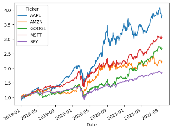
Let’s compare not the price, but the relative performance.
[95]:
df = df['Close']
df = df / df.iloc[0]
df
[95]:
| Ticker | AAPL | AMZN | GOOGL | MSFT | SPY |
|---|---|---|---|---|---|
| Date | |||||
| 2019-01-02 | 1.000000 | 1.000000 | 1.000000 | 1.000000 | 1.000000 |
| 2019-01-03 | 0.900393 | 0.974759 | 0.972304 | 0.963212 | 0.976137 |
| 2019-01-04 | 0.938830 | 1.023559 | 1.022177 | 1.008010 | 1.008834 |
| 2019-01-07 | 0.936740 | 1.058722 | 1.020139 | 1.009296 | 1.016788 |
| 2019-01-08 | 0.954598 | 1.076309 | 1.029099 | 1.016614 | 1.026341 |
| ... | ... | ... | ... | ... | ... |
| 2021-09-17 | 3.805408 | 2.249661 | 2.670004 | 3.061107 | 1.849226 |
| 2021-09-20 | 3.724121 | 2.180277 | 2.630551 | 3.004247 | 1.818391 |
| 2021-09-21 | 3.736886 | 2.172416 | 2.636496 | 3.009351 | 1.816673 |
| 2021-09-22 | 3.799937 | 2.196078 | 2.660209 | 3.047937 | 1.834395 |
| 2021-09-23 | 3.825470 | 2.219436 | 2.677893 | 3.057941 | 1.856683 |
688 rows × 5 columns
[96]:
df.plot()
[96]:
<Axes: xlabel='Date'>
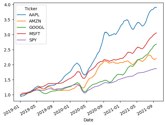
The rolling function will play very nicely with datetime data as shown here when I get the moving average over a 40 day period. And this can handle unevenly sampled date easily.
[97]:
df.rolling('40D').mean().plot()
[97]:
<Axes: xlabel='Date'>
Indexing with datetime data though will require a slightly extra step, but then it is easy.
[98]:
from datetime import date
start = date(2021, 4, 1)
end = date(2021, 4, 30)
[99]:
df[start:end]
[99]:
| Ticker | AAPL | AMZN | GOOGL | MSFT | SPY |
|---|---|---|---|---|---|
| Date | |||||
| 2021-04-01 | 3.194389 | 2.053758 | 2.019361 | 2.463520 | 1.667523 |
| 2021-04-05 | 3.269704 | 2.096464 | 2.103918 | 2.531830 | 1.691457 |
| 2021-04-06 | 3.277755 | 2.094573 | 2.094720 | 2.519530 | 1.690458 |
| 2021-04-07 | 3.321645 | 2.130678 | 2.122947 | 2.540267 | 1.692414 |
| 2021-04-08 | 3.385533 | 2.143614 | 2.133756 | 2.574320 | 1.700448 |
| 2021-04-09 | 3.454095 | 2.190978 | 2.152947 | 2.600749 | 1.712810 |
| 2021-04-12 | 3.408387 | 2.195650 | 2.128247 | 2.601359 | 1.713435 |
| 2021-04-13 | 3.491233 | 2.209040 | 2.137549 | 2.627586 | 1.718512 |
| 2021-04-14 | 3.428904 | 2.165509 | 2.125678 | 2.598107 | 1.712643 |
| 2021-04-15 | 3.493051 | 2.195455 | 2.166771 | 2.637852 | 1.731042 |
| 2021-04-16 | 3.484221 | 2.208676 | 2.164400 | 2.650457 | 1.736827 |
| 2021-04-19 | 3.501882 | 2.190855 | 2.171047 | 2.630127 | 1.728294 |
| 2021-04-20 | 3.456953 | 2.166607 | 2.160854 | 2.625248 | 1.715641 |
| 2021-04-21 | 3.467081 | 2.184364 | 2.160229 | 2.648831 | 1.731874 |
| 2021-04-22 | 3.426567 | 2.149942 | 2.135738 | 2.614168 | 1.716056 |
| 2021-04-23 | 3.488377 | 2.170629 | 2.180690 | 2.654625 | 1.734663 |
| 2021-04-26 | 3.498765 | 2.214888 | 2.190171 | 2.658691 | 1.738284 |
| 2021-04-27 | 3.490195 | 2.220365 | 2.172204 | 2.662960 | 1.737909 |
| 2021-04-28 | 3.469159 | 2.247049 | 2.236735 | 2.587636 | 1.737410 |
| 2021-04-29 | 3.466561 | 2.255372 | 2.268707 | 2.566798 | 1.748482 |
| 2021-04-30 | 3.414101 | 2.252844 | 2.231482 | 2.563443 | 1.736994 |
[100]:
pd.date_range(start='1/1/2019', end='08/31/2021', freq='M')
/tmp/ipykernel_346054/3907196692.py:1: FutureWarning: 'M' is deprecated and will be removed in a future version, please use 'ME' instead.
  pd.date_range(start='1/1/2019', end='08/31/2021', freq='M')
[100]:
DatetimeIndex(['2019-01-31', '2019-02-28', '2019-03-31', '2019-04-30',
               '2019-05-31', '2019-06-30', '2019-07-31', '2019-08-31',
               '2019-09-30', '2019-10-31', '2019-11-30', '2019-12-31',
               '2020-01-31', '2020-02-29', '2020-03-31', '2020-04-30',
               '2020-05-31', '2020-06-30', '2020-07-31', '2020-08-31',
               '2020-09-30', '2020-10-31', '2020-11-30', '2020-12-31',
               '2021-01-31', '2021-02-28', '2021-03-31', '2021-04-30',
               '2021-05-31', '2021-06-30', '2021-07-31', '2021-08-31'],
              dtype='datetime64[ns]', freq='ME')
[101]:
df.resample(rule='Q').max()
/tmp/ipykernel_346054/2442371637.py:1: FutureWarning: 'Q' is deprecated and will be removed in a future version, please use 'QE' instead.
  df.resample(rule='Q').max()
[101]:
| Ticker | AAPL | AMZN | GOOGL | MSFT | SPY |
|---|---|---|---|---|---|
| Date | |||||
| 2019-03-31 | 1.240671 | 1.182005 | 1.172043 | 1.193962 | 1.143114 |
| 2019-06-30 | 1.346620 | 1.275045 | 1.228998 | 1.373424 | 1.187798 |
| 2019-09-30 | 1.435250 | 1.313073 | 1.181344 | 1.410902 | 1.218385 |
| 2019-12-31 | 1.887425 | 1.214842 | 1.291832 | 1.595238 | 1.315273 |
| 2020-03-31 | 2.108058 | 1.410030 | 1.445813 | 1.893692 | 1.377995 |
| 2020-06-30 | 2.367842 | 1.796086 | 1.388762 | 2.053599 | 1.324073 |
| 2020-09-30 | 3.473548 | 2.294446 | 1.628352 | 2.343208 | 1.471860 |
| 2020-12-31 | 3.544630 | 2.237387 | 1.730354 | 2.281494 | 1.551180 |
| 2021-03-31 | 3.712410 | 2.196046 | 2.008780 | 2.484634 | 1.649707 |
| 2021-06-30 | 3.562981 | 2.277547 | 2.323662 | 2.765188 | 1.787611 |
| 2021-09-30 | 4.082359 | 2.424363 | 2.753735 | 3.115720 | 1.892556 |
Sorting & Filtering on Tabular Data
To highlight filtering in DataFrames, we’ll use a dataset with a bunch of different columns/series of different types. This data was pulled directly from the enDAQ cloud API off some example recording files.
[102]:
df = pd.read_csv('https://info.endaq.com/hubfs/data/endaq-cloud-table.csv')
df
[102]:
| Unnamed: 0 | tags | id | serial_number_id | file_name | file_size | recording_length | recording_ts | created_ts | modified_ts | ... | psdResultantOctave | samplePeakWindow | temperatureMeanFull | accelerometerSampleRateFull | psdPeakOctaves | microphonoeRMSFull | gyroscopeRMSFull | pvssResultantOctave | accelerationRMSFull | psdResultant1Hz | |
|---|---|---|---|---|---|---|---|---|---|---|---|---|---|---|---|---|---|---|---|---|---|
| 0 | 0 | ['Vibration Severity: High', 'Shock Severity: ... | 6cd65b8f-1187-3bf9-a431-35304a7f84b7 | 9695 | train-passing-1632515146.ide | 10492602 | 73.612335 | 1588184436 | 1632515146 | 1632515146 | ... | [0. 0. 0.001 0.024 0.032 0.008 0.008 0.0... | [1.241 1.682 1.944 ... 1.852 1.372 1.473] | 23.432 | 19999.0 | [0. 0. 0.001 0.131 0.229 0.045 0.05 0.0... | NaN | 0.625 | [ 10.333 25.952 30.28 52.579 172.174 275.8... | 0.372 | [0. 0. 0. ... 0. 0. 0.] |
| 1 | 1 | ['Vibration Severity: Low', 'Acceleration Seve... | 342aacc3-cd91-3124-8cf4-0c7fece6dcab | 9316 | Seat-Top_09-1632515145.ide | 10491986 | 172.704559 | 1575800071 | 1632515146 | 1632515146 | ... | [0. 0. 0. 0. 0. 0. 0. 0. ... | [0.035 0.024 0.007 ... 0.067 0.031 0.022] | 20.133 | 3996.0 | [0. 0. 0.001 0. 0.001 0. 0.001 0.0... | NaN | 0.945 | [53.648 76.9 43.779 44.217 39.351 11.396 9.... | 0.082 | [ 0. 0. 0. ... nan nan nan] |
| 2 | 2 | ['Shock Severity: Very Low', 'Acceleration Sev... | 5c5592b4-2dbc-3124-be8f-c7179eecda49 | 10118 | Bolted-1632515144.ide | 6149229 | 29.396118 | 1619041447 | 1632515144 | 1632515144 | ... | [0.001 0.003 0.004 0.064 0.106 0.102 0.103 0.1... | [5.283 5.944 5.19 ... 0.356 1.079 1.099] | 23.172 | 20000.0 | [0.001 0.004 0.004 0.128 0.125 0.119 0.14 0.1... | 25.507 | NaN | [ 26.338 27.636 64.097 102.733 107.863 124.6... | 2.398 | [0. 0.001 0.002 ... 0.002 0.001 0.001] |
| 3 | 3 | ['Shock Severity: Very Low', 'Acceleration Sev... | ef832e45-50fa-38b4-8f2c-91769f7cef6e | 10309 | RMI-2000-1632515143.ide | 5909632 | 60.250855 | 24 | 1632515143 | 1632515143 | ... | [0. 0. 0. 0. 0.001 0.002 0.002 0.0... | [0.13 0.118 0.1 ... 0.105 0.1 0.066] | 21.806 | 4012.0 | [0. 0. 0. 0. 0.008 0.01 0.019 0.0... | 1.754 | 1.557 | [ 0.854 1.159 1.662 1.815 3.022 6.139 10.... | 0.079 | [ 0. 0. 0. ... nan nan nan] |
| 4 | 4 | ['Shock Severity: Very Low', 'Acceleration Sev... | 0396df6a-56b0-3e43-8e46-e1d0d7485ff5 | 9295 | Seat-Base_21-1632515142.ide | 5248836 | 83.092255 | 1575800210 | 1632515143 | 1632515143 | ... | [0.002 0.007 0.008 0.005 0.002 0.005 0.002 0.0... | [0.084 0.137 0.178 ... 0.347 0.324 0.286] | 17.820 | 4046.0 | [0.002 0.014 0.016 0.013 0.003 0.031 0.003 0.0... | NaN | 2.666 | [ 74.73 79.453 101.006 151.429 73.92 53.4... | 0.130 | [0.001 0.002 0.002 ... nan nan nan] |
| 5 | 5 | ['Drive-Test', 'Vibration Severity: Very Low',... | 5e293d65-c9e0-3aa1-9098-c9762e8fbc86 | 11046 | Drive-Home_01-1632515142.ide | 3632799 | 61.755371 | 1616178955 | 1632515142 | 1632515142 | ... | [0. 0. 0. 0. 0.001 0. 0. 0. ... | [0.001 0.003 0.002 ... 0.011 0.008 0.006] | 29.061 | 4013.0 | [0. 0. 0. 0. 0.007 0. 0. 0. ... | 16.243 | 0.363 | [ 2.336 7.82 19.078 10.384 16.975 38.326 18.... | 0.021 | [ 0. 0. 0. ... nan nan nan] |
| 6 | 6 | ['Acceleration Severity: High', 'Shock Severit... | cd81c850-9e22-3b20-b570-7411e7a144cc | 0 | HiTest-Shock-1632515141.ide | 2655894 | 20.331848 | 1543936974 | 1632515141 | 1632515141 | ... | [0.304 0.486 0.399 0.454 0.347 0.178 0.185 0.1... | [ 3.088 3.019 2.893 ... 73.794 40.005 24.303] | 9.538 | 19997.0 | [ 0.304 0.537 0.479 0.811 0.624 0.554 0.... | NaN | NaN | [1378.444 2470.941 4368.78 5033.327 5814.49 ... | 11.645 | [0.157 0.304 0.42 ... 0.001 0.01 0.013] |
| 7 | 7 | ['Vibration Severity: High', 'Acceleration Sev... | 0931a23d-3515-3d11-bf97-bb9b2c7863be | 11162 | Calibration-Shake-1632515140.IDE | 2218130 | 27.882690 | 1621278970 | 1632515140 | 1632515140 | ... | [2.100e-02 7.400e-02 7.500e-02 4.900e-02 5.500... | [7.486 7.496 7.137 ... 7.997 8.294 7.806] | 24.545 | 5000.0 | [2.10000e-02 9.00000e-02 8.60000e-02 6.30000e-... | NaN | 0.166 | [ 90.703 198.651 288.078 183.492 126.417 108.4... | 2.712 | [0.007 0.021 0.055 ... nan nan nan] |
| 8 | 8 | ['Shock Severity: Very Low', 'Acceleration Sev... | c1571d10-2329-3aea-aa5d-223733f6336b | 10916 | FUSE_HSTAB_000005-1632515139.ide | 537562 | 18.491791 | 1619108004 | 1632515140 | 1632515140 | ... | [ 0. 0. 0. 0. 0. 0. 0. nan nan nan nan n... | [0.001 0.001 0.001 ... 0.002 0.006 0.006] | 18.874 | 504.0 | [0. 0. 0.001 0.001 0. 0. 0. n... | NaN | 0.749 | [ 2.617 6.761 17.326 34.067 28.721 9.469 15.... | 0.011 | [ 0. 0. 0. ... nan nan nan] |
| 9 | 0 | ['Shock Severity: Medium', 'Acceleration Sever... | 8ce137ff-904e-314b-81ff-ff2cea279db2 | 9874 | Coffee_002-1631722736.IDE | 60959516 | 769.299896 | 952113744 | 1631722736 | 1631722736 | ... | [] | [] | 24.540 | 5000.0 | [] | NaN | 0.082 | [] | 0.059 | [] |
| 10 | 1 | ['Vibration Severity: High', 'Shock Severity: ... | 9d7383fb-40d6-34c1-9d0c-37f11c29bff5 | 11456 | 100_Joules_900_lbs-1629315313.ide | 1596714 | 20.200623 | 1627327315 | 1629315313 | 1629315313 | ... | [0.071 0.201 0.293 0.686 1.565 1.028 0.856 0.9... | [0.304 0.274 0.296 ... 1.513 1.313 0.652] | 24.180 | 5000.0 | [0.071 0.236 0.311 1.148 2.036 1.791 1.498 2.7... | NaN | 24.471 | [ 194.741 361.14 563.488 855.34 1712.229 ... | 2.877 | [0.02 0.071 0.138 ... nan nan nan] |
| 11 | 2 | ['Acceleration Severity: High', 'Shock Severit... | 5f35ed7f-ff55-36a3-896d-276f06a0e340 | 11456 | 50_Joules_900_lbs-1629315312.ide | 1597750 | 20.201752 | 1627329399 | 1629315312 | 1629315312 | ... | [0.074 0.196 0.327 0.874 1.521 0.917 0.478 0.7... | [0.304 0.21 0.098 ... 0.693 1.418 0.932] | 24.175 | 5000.0 | [0.074 0.232 0.392 1.258 2.045 2.049 1.143 2.3... | NaN | 15.575 | [ 242.141 388.517 736.981 1070.284 1843.722 ... | 2.423 | [0.021 0.074 0.137 ... nan nan nan] |
| 12 | 3 | ['Shock Severity: Very Low', 'Vibration Severi... | f7240576-47c6-34b8-bdce-3fe11bb5f1c6 | 11046 | Drive-Home_07-1626805222.ide | 36225758 | 634.732056 | 1616182557 | 1626805222 | 1626805222 | ... | [] | [] | 28.832 | 4012.0 | [] | 16.277 | 4.185 | [] | 0.097 | [] |
| 13 | 4 | ['Big-Mining'] | c2c234cc-8055-3fba-ad8b-446c4b6f85dc | 5120 | Mining-SSX28803_06-1626457584.IDE | 402920686 | 3238.119202 | 1536953304 | 1626457585 | 1626457585 | ... | [] | [] | NaN | NaN | [] | NaN | NaN | [] | NaN | [] |
| 14 | 5 | ['Shock Severity: Medium', 'Acceleration Sever... | 69fd99f8-3d85-38ec-9f5d-67e9d7b7e868 | 10030 | 200922_Moto_Max_Run5_Control_Larry-1626297441.ide | 4780893 | 99.325134 | 1600818455 | 1626297442 | 1626297442 | ... | [0. 0. 0. 0. 0. 0. 0. 0. 0. 0. 0. 0. 0.] | [ 3.34 13.586 10.13 ... 7.737 8.978 8.672] | NaN | 4014.0 | [[0. 0. 0. 0. 0. 0. 0. 0. 0. 0. 0. 0. 0.]\n [0... | NaN | NaN | [165.983 278.352 717.331 950.513 697.421 358.6... | 3.528 | [0.006 0.016 0.04 ... nan nan nan] |
| 15 | 6 | ['Ford'] | f38361de-30a7-3dda-aec4-e87a67d1ecbb | 9695 | ford_f150-1626296561.ide | 96097059 | 1207.678344 | 1584142508 | 1626296561 | 1626296561 | ... | [] | [] | NaN | NaN | [] | NaN | NaN | [] | NaN | [] |
| 16 | 7 | ['Shock Severity: High', 'Vibration Severity: ... | 40718e01-f422-3926-a22d-acf6daf1182b | 7530 | Motorcycle-Car-Crash-1626277852.ide | 10489262 | 151.069336 | 1562173372 | 1626277852 | 1626277852 | ... | [0. 0. 0. 0. 0. 0. 0. 0. 0. 0. 0. 0. 0.] | [3.371 3.641 3.649 ... 6.168 7.463 7.04 ] | 26.989 | 10001.0 | [[0. 0. 0. 0. 0. 0. 0. 0. 0. 0. 0. 0. 0.]\n [0... | NaN | 19.810 | [ 2723.153 5977.212 11406.291 12031.397 7337... | 1.732 | [2.250e-01 8.390e-01 2.025e+00 ... 1.000e-03 1... |
| 17 | 8 | ['Shock Severity: Very Low', 'Surgical', 'Vibr... | ee6dc613-d422-347c-8119-f122a55ac81a | 11071 | surgical-instrument-1625829182.ide | 541994 | 6.951172 | 1619110390 | 1625829183 | 1625829183 | ... | [0. 0. 0. 0. 0. 0. 0. 0. 0. 0. 0. 0. 0.] | [0.667 0.549 1.05 ... 1.109 2.86 3.99 ] | 21.889 | 5000.0 | [[0. 0. 0. 0. 0. 0. 0. 0. 0. 0. 0. 0. 0.]\n [0... | NaN | 4.647 | [ 88.953 171.73 104.303 71.184 58.883 72.4... | 1.568 | [0.001 0.001 0.003 ... nan nan nan] |
| 18 | 9 | ['Acceleration Severity: High', 'Shock Severit... | f642d81c-7fe7-37fd-ab75-d493fc0556db | 9680 | LOC__3__DAQ41551_11_01_02-1625170795.IDE | 2343292 | 28.456818 | 1616645179 | 1625170795 | 1625170795 | ... | [0. 0. 0. 0. 0. 0. 0. 0. 0. 0. 0. 0. 0.] | [ 32.679 24.925 30.95 ... 106.511 27.715 ... | 33.452 | 20010.0 | [[0. 0. 0. 0. 0. 0. 0. 0. 0. 0. 0. 0. 0.]\n [0... | NaN | 286.217 | [2333.993 5629.021 6417.48 5802.895 3692.838 ... | 94.197 | [ 2.09 8.631 18.196 ... 69.565 59.225 60.801] |
| 19 | 10 | ['Vibration Severity: High', 'Shock Severity: ... | 0c0e92ae-214a-32bd-a5bb-5e1801da06b2 | 9680 | LOC__4__DAQ41551_15_05-1625170794.IDE | 6927958 | 64.486054 | 1616646130 | 1625170794 | 1625170794 | ... | [0. 0. 0. 0. 0. 0. 0. 0. 0. 0. 0. 0. 0.] | [14.223 14.903 24.949 ... 11.482 21.319 32.766] | 32.202 | 19992.0 | [[0. 0. 0. 0. 0. 0. 0. 0. 0. 0. 0. 0. 0.]\n [0... | NaN | 277.654 | [ 378.188 748.336 1054.232 1115.369 756.905 ... | 46.528 | [ 0.072 0.302 0.816 ... 52.226 45.804 52.81 ] |
| 20 | 11 | ['Vibration Severity: High', 'Mining-Hammer', ... | 99ac47a8-63c2-38a4-8d92-508698eb3752 | 9680 | LOC__6__DAQ41551_25_01-1625170793.IDE | 8664238 | 63.878937 | 1616648007 | 1625170793 | 1625170793 | ... | [0. 0. 0. 0. 0. 0. 0. 0. 0. 0. 0. 0. 0.] | [ 66.83 54.723 63.536 ... 109.259 85.341 ... | 26.031 | 19992.0 | [[0. 0. 0. 0. 0. 0. 0. 0. 0. 0. 0. 0. 0.]\n [0... | NaN | 245.929 | [ 780.577 1168.663 1851.417 1094.945 793.122 ... | 54.408 | [ 0.162 0.587 1.495 ... 45.639 43.86 40.177] |
| 21 | 12 | ['Mining-Hammer', 'Vibration Severity: High', ... | ebf31fb2-9d36-37de-999c-3edb01f17fb2 | 9680 | LOC__2__DAQ38060_06_03_05-1625170793.IDE | 1519172 | 27.057647 | 1616640862 | 1625170793 | 1625170793 | ... | [0. 0. 0. 0. 0. 0. 0. 0. 0. 0. 0. 0. 0.] | [ 33.294 29.392 19.99 ... 175.123 162.043 ... | 25.616 | 19998.0 | [[0. 0. 0. 0. 0. 0. 0. 0. 0. 0. 0. 0. 0.]\n [0... | NaN | 266.815 | [1073.684 940.873 1063.151 957.568 975.826 ... | 131.087 | [ 0.371 0.409 0.787 ... 27.577 24.778 37.822] |
| 22 | 13 | ['Shock Severity: Very Low', 'Vibration Severi... | e39fe506-f39a-3301-866c-9da6a30f9577 | 9695 | Tilt_000000-1625156721.IDE | 719403 | 23.355163 | 1625156461 | 1625156722 | 1625156722 | ... | [0. 0. 0. 0. 0. 0. 0. 0. 0. 0. 0. 0. 0.] | [0.033 0.029 0.03 ... nan nan nan] | 26.410 | 5000.0 | [[0. 0. 0. 0. 0. 0. 0. 0. 0. 0. 0. 0. 0.]\n [0... | NaN | 11.933 | [142.046 273.02 216.774 129.288 54.011 24.0... | 0.044 | [0.008 0.02 0.03 ... nan nan nan] |
23 rows × 29 columns
[103]:
df.columns
[103]:
Index(['Unnamed: 0', 'tags', 'id', 'serial_number_id', 'file_name',
       'file_size', 'recording_length', 'recording_ts', 'created_ts',
       'modified_ts', 'device', 'gpsLocationFull', 'velocityRMSFull',
       'gpsSpeedFull', 'pressureMeanFull', 'samplePeakStartTime',
       'displacementRMSFull', 'psuedoVelocityPeakFull', 'accelerationPeakFull',
       'psdResultantOctave', 'samplePeakWindow', 'temperatureMeanFull',
       'accelerometerSampleRateFull', 'psdPeakOctaves', 'microphonoeRMSFull',
       'gyroscopeRMSFull', 'pvssResultantOctave', 'accelerationRMSFull',
       'psdResultant1Hz'],
      dtype='object')
There’s a lot of data here! So we’ll focus on just a handful of columns and convert the time in seconds to a datetime object.
[104]:
df = df[['serial_number_id', 'file_name', 'file_size', 'recording_length', 'recording_ts',
         'accelerationPeakFull', 'psuedoVelocityPeakFull', 'accelerationRMSFull',
         'velocityRMSFull', 'displacementRMSFull', 'pressureMeanFull', 'temperatureMeanFull']].copy()

df['recording_ts'] = pd.to_datetime(df['recording_ts'], unit='s')
df = df.sort_values(by=['recording_ts'], ascending=False)
df
[104]:
| serial_number_id | file_name | file_size | recording_length | recording_ts | accelerationPeakFull | psuedoVelocityPeakFull | accelerationRMSFull | velocityRMSFull | displacementRMSFull | pressureMeanFull | temperatureMeanFull | |
|---|---|---|---|---|---|---|---|---|---|---|---|---|
| 11 | 11456 | 50_Joules_900_lbs-1629315312.ide | 1597750 | 20.201752 | 2021-07-26 19:56:39 | 231.212 | 2907.650 | 2.423 | 54.507 | 1.066 | 98.745 | 24.175 |
| 10 | 11456 | 100_Joules_900_lbs-1629315313.ide | 1596714 | 20.200623 | 2021-07-26 19:21:55 | 218.634 | 2961.256 | 2.877 | 53.875 | 1.053 | 98.751 | 24.180 |
| 22 | 9695 | Tilt_000000-1625156721.IDE | 719403 | 23.355163 | 2021-07-01 16:21:01 | 0.378 | 330.946 | 0.044 | 11.042 | 0.345 | 99.510 | 26.410 |
| 7 | 11162 | Calibration-Shake-1632515140.IDE | 2218130 | 27.882690 | 2021-05-17 19:16:10 | 8.783 | 1142.282 | 2.712 | 46.346 | 0.617 | 102.251 | 24.545 |
| 17 | 11071 | surgical-instrument-1625829182.ide | 541994 | 6.951172 | 2021-04-22 16:53:10 | 5.739 | 387.312 | 1.568 | 24.418 | 0.242 | 99.879 | 21.889 |
| 8 | 10916 | FUSE_HSTAB_000005-1632515139.ide | 537562 | 18.491791 | 2021-04-22 16:13:24 | 0.202 | 53.375 | 0.011 | 1.504 | 0.036 | 90.706 | 18.874 |
| 2 | 10118 | Bolted-1632515144.ide | 6149229 | 29.396118 | 2021-04-21 21:44:07 | 15.343 | 148.276 | 2.398 | 14.101 | 0.154 | 99.652 | 23.172 |
| 20 | 9680 | LOC__6__DAQ41551_25_01-1625170793.IDE | 8664238 | 63.878937 | 2021-03-25 04:53:27 | 564.966 | 2357.599 | 54.408 | 145.223 | 3.088 | 102.875 | 26.031 |
| 19 | 9680 | LOC__4__DAQ41551_15_05-1625170794.IDE | 6927958 | 64.486054 | 2021-03-25 04:22:10 | 585.863 | 2153.020 | 46.528 | 148.591 | 2.615 | 105.750 | 32.202 |
| 18 | 9680 | LOC__3__DAQ41551_11_01_02-1625170795.IDE | 2343292 | 28.456818 | 2021-03-25 04:06:19 | 622.040 | 8907.949 | 94.197 | 372.049 | 9.580 | 105.682 | 33.452 |
| 21 | 9680 | LOC__2__DAQ38060_06_03_05-1625170793.IDE | 1519172 | 27.057647 | 2021-03-25 02:54:22 | 995.670 | 5845.241 | 131.087 | 323.287 | 3.144 | 104.473 | 25.616 |
| 12 | 11046 | Drive-Home_07-1626805222.ide | 36225758 | 634.732056 | 2021-03-19 19:35:57 | 23.805 | 356.128 | 0.097 | 6.117 | 0.135 | 101.988 | 28.832 |
| 5 | 11046 | Drive-Home_01-1632515142.ide | 3632799 | 61.755371 | 2021-03-19 18:35:55 | 0.479 | 40.197 | 0.021 | 1.081 | 0.023 | 100.284 | 29.061 |
| 14 | 10030 | 200922_Moto_Max_Run5_Control_Larry-1626297441.ide | 4780893 | 99.325134 | 2020-09-22 23:47:35 | 29.864 | 1280.349 | 3.528 | 55.569 | 1.060 | NaN | NaN |
| 0 | 9695 | train-passing-1632515146.ide | 10492602 | 73.612335 | 2020-04-29 18:20:36 | 7.513 | 419.944 | 0.372 | 6.969 | 0.061 | 104.620 | 23.432 |
| 15 | 9695 | ford_f150-1626296561.ide | 96097059 | 1207.678344 | 2020-03-13 23:35:08 | NaN | NaN | NaN | NaN | NaN | NaN | NaN |
| 4 | 9295 | Seat-Base_21-1632515142.ide | 5248836 | 83.092255 | 2019-12-08 10:16:50 | 1.085 | 251.009 | 0.130 | 7.318 | 0.190 | 98.930 | 17.820 |
| 1 | 9316 | Seat-Top_09-1632515145.ide | 10491986 | 172.704559 | 2019-12-08 10:14:31 | 1.105 | 86.595 | 0.082 | 1.535 | 0.040 | 98.733 | 20.133 |
| 16 | 7530 | Motorcycle-Car-Crash-1626277852.ide | 10489262 | 151.069336 | 2019-07-03 17:02:52 | 480.737 | 12831.590 | 1.732 | 143.437 | 3.988 | 100.363 | 26.989 |
| 6 | 0 | HiTest-Shock-1632515141.ide | 2655894 | 20.331848 | 2018-12-04 15:22:54 | 619.178 | 6058.093 | 11.645 | 167.835 | 4.055 | 101.126 | 9.538 |
| 13 | 5120 | Mining-SSX28803_06-1626457584.IDE | 402920686 | 3238.119202 | 2018-09-14 19:28:24 | NaN | NaN | NaN | NaN | NaN | NaN | NaN |
| 9 | 9874 | Coffee_002-1631722736.IDE | 60959516 | 769.299896 | 2000-03-03 20:02:24 | 2.698 | 1338.396 | 0.059 | 5.606 | 0.104 | 100.339 | 24.540 |
| 3 | 10309 | RMI-2000-1632515143.ide | 5909632 | 60.250855 | 1970-01-01 00:00:24 | 0.332 | 17.287 | 0.079 | 1.247 | 0.005 | 100.467 | 21.806 |
Filtering is made simple with boolean expressions that can be combined. There is also a method to sort_values by columns/series.
[105]:
mask = df.recording_ts > pd.to_datetime('2021-01-01')
df[mask].sort_values(by=['serial_number_id'], ascending=False)
[105]:
| serial_number_id | file_name | file_size | recording_length | recording_ts | accelerationPeakFull | psuedoVelocityPeakFull | accelerationRMSFull | velocityRMSFull | displacementRMSFull | pressureMeanFull | temperatureMeanFull | |
|---|---|---|---|---|---|---|---|---|---|---|---|---|
| 11 | 11456 | 50_Joules_900_lbs-1629315312.ide | 1597750 | 20.201752 | 2021-07-26 19:56:39 | 231.212 | 2907.650 | 2.423 | 54.507 | 1.066 | 98.745 | 24.175 |
| 10 | 11456 | 100_Joules_900_lbs-1629315313.ide | 1596714 | 20.200623 | 2021-07-26 19:21:55 | 218.634 | 2961.256 | 2.877 | 53.875 | 1.053 | 98.751 | 24.180 |
| 7 | 11162 | Calibration-Shake-1632515140.IDE | 2218130 | 27.882690 | 2021-05-17 19:16:10 | 8.783 | 1142.282 | 2.712 | 46.346 | 0.617 | 102.251 | 24.545 |
| 17 | 11071 | surgical-instrument-1625829182.ide | 541994 | 6.951172 | 2021-04-22 16:53:10 | 5.739 | 387.312 | 1.568 | 24.418 | 0.242 | 99.879 | 21.889 |
| 12 | 11046 | Drive-Home_07-1626805222.ide | 36225758 | 634.732056 | 2021-03-19 19:35:57 | 23.805 | 356.128 | 0.097 | 6.117 | 0.135 | 101.988 | 28.832 |
| 5 | 11046 | Drive-Home_01-1632515142.ide | 3632799 | 61.755371 | 2021-03-19 18:35:55 | 0.479 | 40.197 | 0.021 | 1.081 | 0.023 | 100.284 | 29.061 |
| 8 | 10916 | FUSE_HSTAB_000005-1632515139.ide | 537562 | 18.491791 | 2021-04-22 16:13:24 | 0.202 | 53.375 | 0.011 | 1.504 | 0.036 | 90.706 | 18.874 |
| 2 | 10118 | Bolted-1632515144.ide | 6149229 | 29.396118 | 2021-04-21 21:44:07 | 15.343 | 148.276 | 2.398 | 14.101 | 0.154 | 99.652 | 23.172 |
| 22 | 9695 | Tilt_000000-1625156721.IDE | 719403 | 23.355163 | 2021-07-01 16:21:01 | 0.378 | 330.946 | 0.044 | 11.042 | 0.345 | 99.510 | 26.410 |
| 19 | 9680 | LOC__4__DAQ41551_15_05-1625170794.IDE | 6927958 | 64.486054 | 2021-03-25 04:22:10 | 585.863 | 2153.020 | 46.528 | 148.591 | 2.615 | 105.750 | 32.202 |
| 20 | 9680 | LOC__6__DAQ41551_25_01-1625170793.IDE | 8664238 | 63.878937 | 2021-03-25 04:53:27 | 564.966 | 2357.599 | 54.408 | 145.223 | 3.088 | 102.875 | 26.031 |
| 21 | 9680 | LOC__2__DAQ38060_06_03_05-1625170793.IDE | 1519172 | 27.057647 | 2021-03-25 02:54:22 | 995.670 | 5845.241 | 131.087 | 323.287 | 3.144 | 104.473 | 25.616 |
| 18 | 9680 | LOC__3__DAQ41551_11_01_02-1625170795.IDE | 2343292 | 28.456818 | 2021-03-25 04:06:19 | 622.040 | 8907.949 | 94.197 | 372.049 | 9.580 | 105.682 | 33.452 |
[106]:
mask = (df.recording_ts > pd.to_datetime('2021-01-01')) & (df.accelerationPeakFull > 100)
df[mask].sort_values(by=['accelerationPeakFull'], ascending=False)
[106]:
| serial_number_id | file_name | file_size | recording_length | recording_ts | accelerationPeakFull | psuedoVelocityPeakFull | accelerationRMSFull | velocityRMSFull | displacementRMSFull | pressureMeanFull | temperatureMeanFull | |
|---|---|---|---|---|---|---|---|---|---|---|---|---|
| 21 | 9680 | LOC__2__DAQ38060_06_03_05-1625170793.IDE | 1519172 | 27.057647 | 2021-03-25 02:54:22 | 995.670 | 5845.241 | 131.087 | 323.287 | 3.144 | 104.473 | 25.616 |
| 18 | 9680 | LOC__3__DAQ41551_11_01_02-1625170795.IDE | 2343292 | 28.456818 | 2021-03-25 04:06:19 | 622.040 | 8907.949 | 94.197 | 372.049 | 9.580 | 105.682 | 33.452 |
| 19 | 9680 | LOC__4__DAQ41551_15_05-1625170794.IDE | 6927958 | 64.486054 | 2021-03-25 04:22:10 | 585.863 | 2153.020 | 46.528 | 148.591 | 2.615 | 105.750 | 32.202 |
| 20 | 9680 | LOC__6__DAQ41551_25_01-1625170793.IDE | 8664238 | 63.878937 | 2021-03-25 04:53:27 | 564.966 | 2357.599 | 54.408 | 145.223 | 3.088 | 102.875 | 26.031 |
| 11 | 11456 | 50_Joules_900_lbs-1629315312.ide | 1597750 | 20.201752 | 2021-07-26 19:56:39 | 231.212 | 2907.650 | 2.423 | 54.507 | 1.066 | 98.745 | 24.175 |
| 10 | 11456 | 100_Joules_900_lbs-1629315313.ide | 1596714 | 20.200623 | 2021-07-26 19:21:55 | 218.634 | 2961.256 | 2.877 | 53.875 | 1.053 | 98.751 | 24.180 |
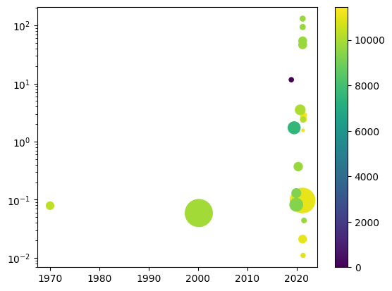
Another preview to plotly, but visualizing dataframes is made easy, even with mixed types.
[107]:
fig, ax = plt.subplots()
scatter = ax.scatter(df['recording_ts'],
                     df['accelerationRMSFull'],
                     s=df['recording_length'],
                     c=df['serial_number_id'],
                     cmap='viridis')
plt.colorbar(scatter)
plt.yscale('log')
plt.show()
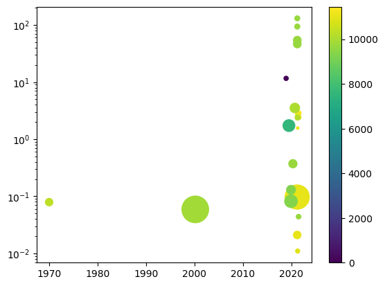
Plotly automatically made my colors a colorbar because I specified it based on a numeric value. If instead I change the type to string and replot, we’ll see discrete series for each device.
[108]:
df['device'] = df["serial_number_id"].astype(str)

fig, ax = plt.subplots()

scatter = ax.scatter(df['recording_ts'],
                     df['accelerationRMSFull'],
                     s=df['recording_length'],
                     c=df['serial_number_id'],
                     cmap='viridis')

plt.colorbar(scatter)
plt.yscale('log')
plt.show()