3. 📌 Introduction to PyTorch

Filled notebook:

Author: Benjamin I. Fortuno

This notebook provides a comprehensive introduction to PyTorch, covering: - 🔢 Tensor creation and operations - 📏 Reshaping and slicing - ⚡ Matrix operations - 🎯 Automatic differentiation with autograd - 📈 Visualization of computation graphs

By the end of this notebook, you’ll be comfortable using PyTorch for basic computations and setting up gradients for deep learning models.

Setting Up PyTorch

import torch
import numpy as np
import time

# Check if GPU is available
device = torch.device("cuda" if torch.cuda.is_available() else "cpu")
print(f"Using device: {device}")

Using device: cpu

Creating and Manipulating Tensors

Tensors are similar to NumPy arrays but come with GPU acceleration and automatic differentiation.

# Creating different types of tensors
x = torch.tensor([[1, 2], [3, 4]], dtype=torch.float32, device=device)
y = torch.rand((2,2), device=device)  # Random tensor
z = torch.zeros((3,3), device=device)  # Zero tensor
ones = torch.ones((3,3), device=device)  # Ones tensor

print("Tensor x:", x, "\n")
print("Random Tensor y:", y, "\n")
print("Zero Tensor:", z, "\n")
print("Ones Tensor:", ones)

Tensor x: tensor([[1., 2.],
        [3., 4.]])

Random Tensor y: tensor([[0.7179, 0.9155],
        [0.9773, 0.2281]])

Zero Tensor: tensor([[0., 0., 0.],
        [0., 0., 0.],
        [0., 0., 0.]])

Ones Tensor: tensor([[1., 1., 1.],
        [1., 1., 1.],
        [1., 1., 1.]])

📏 Tensor Shapes and Reshaping

# Reshaping tensors
x_reshaped = x.view(4, 1)  # Change shape to (4,1)
print("Original Shape:", x.shape)
print("Reshaped Tensor:")
print(x_reshaped)

Original Shape: torch.Size([2, 2])
Reshaped Tensor:
tensor([[1.],
        [2.],
        [3.],
        [4.]])

🎭 Indexing and Slicing Tensors

# Indexing tensors
tensor = torch.arange(10)
print("Original Tensor:", tensor)

# Accessing elements
print("First element:", tensor[0])
print("Last element:", tensor[-1])

# Slicing
print("First 5 elements:", tensor[:5])
print("Elements from index 3 to 7:", tensor[3:8])

Original Tensor: tensor([0, 1, 2, 3, 4, 5, 6, 7, 8, 9])
First element: tensor(0)
Last element: tensor(9)
First 5 elements: tensor([0, 1, 2, 3, 4])
Elements from index 3 to 7: tensor([3, 4, 5, 6, 7])

⚡ Matrix Operations

# Matrix multiplication
dot_result = torch.mm(x, x)
print("Matrix Multiplication:")
print(dot_result)

Matrix Multiplication:
tensor([[ 7., 10.],
        [15., 22.]])

🔢 Advanced Tensor Operations

Understanding advanced tensor operations helps in optimizing computations and reducing code complexity.

# Stacking and Concatenation
a = torch.rand((3, 3))                      # Random 3x3 tensor
b = torch.rand((3, 3))                      # Random 3x3 tensor
stacked = torch.stack((a, b))               # Stack along a new dimension
concatenated = torch.cat((a, b), dim=0)     # Concatenate along an existing dimension

print("Stacked Tensor Shape:", stacked.shape)
print("Concatenated Tensor Shape:", concatenated.shape)

Stacked Tensor Shape: torch.Size([2, 3, 3])
Concatenated Tensor Shape: torch.Size([6, 3])

Automatic Differentiation with Autograd

PyTorch’s autograd module enables automatic differentiation for computing gradients in neural networks.

# Defining tensors with gradient tracking
a = torch.tensor([2.0, 3.0], requires_grad=True, device=device)
b = torch.tensor([4.0, 5.0], requires_grad=True, device=device)

# Define function: f = a^2 + b^3
f = a**2 + b**3
print("Function values:")
print(f)

Function values:
tensor([ 68., 134.], grad_fn=<AddBackward0>)

# Compute Gradients
f.backward(torch.tensor([1.0, 1.0], device=device))
print("\nGradients:")
print(f"df/da: {a.grad}")
print(f"df/db: {b.grad}")

Gradients:
df/da: tensor([4., 6.])
df/db: tensor([48., 75.])

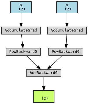
📈 Visualizing Gradients

We can visualize the computation graph and gradients using PyTorch’s torchviz package.

from torchviz import make_dot
from IPython.display import Image

dot_graph = make_dot(f, params={'a': a, 'b': b})  # Create graph
dot_graph.render("computation_graph", format="png")  # Save as PNG

# Display inline in Jupyter
display(Image(filename="computation_graph.png"))

GPU Acceleration

Using GPUs can significantly speed up AI computations, especially when training deep learning models.

# Run this cell if GPU is available
if device == torch.device("cuda"):
    # Comparing CPU vs GPU computation speed
    x_cpu = torch.rand((10000, 10000))
    x_gpu = x_cpu.to(device)

    # Measure time on CPU
    start_cpu = time.time()
    y_cpu = x_cpu * x_cpu
    end_cpu = time.time()

    # Measure time on GPU
    start_gpu = time.time()
    y_gpu = x_gpu * x_gpu
    torch.cuda.synchronize()
    end_gpu = time.time()

    print(f"CPU Time: {end_cpu - start_cpu:.5f} sec")
    print(f"GPU Time: {end_gpu - start_gpu:.5f} sec")

else:
    print("No GPU available. Skipping computation speed comparison.")

No GPU available. Skipping computation speed comparison.

Exercise: Compute Gradients

Task: Define a new function g = 3a^3 + 2b^2 and compute its gradients.

Try implementing this in the cell below!

# TODO: Define g = 3a^3 + 2b^2 and compute gradients

Summary

• ✅ Learned how to create and manipulate tensors

• ✅ Performed basic mathematical operations

• ✅ Explored automatic differentiation with autograd

• ✅ Visualized computation graphs

PyTorch is a powerful tool for deep learning, and mastering these fundamentals will help you in future projects! 🚀